main topic interpreting results session command see also
You are trying to increase the robustness of a measurement system. A measurement system is dynamic because as the input signal changes, the output response changes. Ideally, a measurement system should have a 1:1 correspondence between the value being measured (signal factor) and the measured response (system output). Similarly, zero should serve as the fixed reference point (all lines should be fit through the origin) because an input signal of zero should result in a measurement of zero.
Your initial experiment included seven potential control factors but your results suggested that three factors, each with two levels, are most important: sensor, output device, and relay. The signal factor is the actual value of the item being measured and the output response is the measurement. You have identified two noise conditions.
1 Open the worksheet SENSOR.MTW. The design and response data have been saved for you.
2 Choose Stat > DOE > Taguchi > Analyze Taguchi Design.
3 In Response data are in, enter Noise1 and Noise2.
4 Click Graphs. Under Generate plots of main effects and selected interactions for, check Standard deviations. (Make sure Signal to Noise ratios and Slopes are checked.)
5 Check Display scatterplots with fitted lines. Click OK.
6 Click Analysis. Under Display response tables for, check Standard deviations. (Make sure Signal to Noise ratios and Slopes are checked.)
7 Under Fit linear model for, check Signal to Noise ratios, Slopes, and Standard deviations
8 Click OK in each dialog box.
Session window output
Taguchi Analysis: Noise1, Noise2 versus Sensor, Output, Relay
Linear Model Analysis: SN ratios versus Sensor, Output, Relay
Estimated Model Coefficients for SN ratios
Term Coef SE Coef T P Constant 20.6879 0.3017 68.560 0.000 Sensor 1 2.0050 0.3017 6.645 0.003 Output 1 -0.4724 0.3017 -1.566 0.192 Relay 1 -0.5370 0.3017 -1.780 0.150
S = 0.8535 R-Sq = 92.6% R-Sq(adj) = 87.0%
Analysis of Variance for SN ratios
Source DF Seq SS Adj SS Adj MS F P Sensor 1 32.162 32.162 32.1616 44.15 0.003 Output 1 1.785 1.785 1.7855 2.45 0.192 Relay 1 2.307 2.307 2.3071 3.17 0.150 Residual Error 4 2.914 2.914 0.7284 Total 7 39.168
Linear Model Analysis: Slopes versus Sensor, Output, Relay
Estimated Model Coefficients for Slopes
Term Coef SE Coef T P Constant 1.00122 0.000125 8039.325 0.000 Sensor 1 -0.00034 0.000125 -2.708 0.054 Output 1 0.00004 0.000125 0.294 0.783 Relay 1 0.00003 0.000125 0.274 0.798
S = 0.0003523 R-Sq = 65.2% R-Sq(adj) = 39.1%
Analysis of Variance for Slopes
Source DF Seq SS Adj SS Adj MS F P Sensor 1 0.000001 0.000001 0.000001 7.33 0.054 Output 1 0.000000 0.000000 0.000000 0.09 0.783 Relay 1 0.000000 0.000000 0.000000 0.07 0.798 Residual Error 4 0.000000 0.000000 0.000000 Total 7 0.000001
Linear Model Analysis: StDevs versus Sensor, Output, Relay
Estimated Model Coefficients for StDevs
Term Coef SE Coef T P Constant 0.095414 0.002341 40.753 0.000 Sensor 1 -0.021261 0.002341 -9.081 0.001 Output 1 0.003906 0.002341 1.668 0.171 Relay 1 0.005262 0.002341 2.247 0.088
S = 0.006622 R-Sq = 95.8% R-Sq(adj) = 92.6%
Analysis of Variance for StDevs
Source DF Seq SS Adj SS Adj MS F P Sensor 1 0.003616 0.003616 0.003616 82.46 0.001 Output 1 0.000122 0.000122 0.000122 2.78 0.171 Relay 1 0.000221 0.000221 0.000221 5.05 0.088 Residual Error 4 0.000175 0.000175 0.000044 Total 7 0.004135
Response Table for Signal to Noise Ratios Dynamic Response
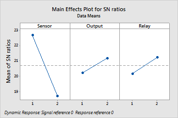
Level Sensor Output Relay 1 22.69 20.22 20.15 2 18.68 21.16 21.22 Delta 4.01 0.94 1.07 Rank 1 3 2
Response Table for Slopes
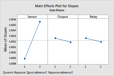
Level Sensor Output Relay 1 1.001 1.001 1.001 2 1.002 1.001 1.001 Delta 0.001 0.000 0.000 Rank 1 2 3
Response Table for Standard Deviations
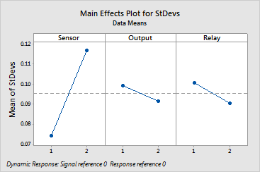
Level Sensor Output Relay 1 0.07415 0.09932 0.10068 2 0.11668 0.09151 0.09015 Delta 0.04252 0.00781 0.01052 Rank 1 3 2 |
Graph window output


Each linear model analysis provides the coefficients for each factor at the low level, their p-values and an analysis of variance table. Use the results to determine whether the factors are significantly related to the response data and each factor's relative importance in the model.
The order of the coefficients by absolute value indicates the relative importance of each factor to the response; the factor with the biggest coefficient has the greatest impact. The sequential and adjusted sums of squares in the analysis of variance table also indicate the relative importance of each factor; the factor with the biggest sum of squares has the greatest impact. These results mirror the factor ranks in the response tables.
In this example, the p-values for the coefficients indicate that sensor is significant in all models at the 0.10 a-level and relay is significant only in the model with standard deviations at the 0.10 a-level.
The response tables show the average of each response characteristic (S/N ratios, means) for each level of each factor. The tables include ranks based on Delta statistics, which compare the relative magnitude of effects. The Delta statistic is the highest minus the lowest average for each factor. Minitab assigns ranks based on Delta values; rank 1 to the highest Delta value, rank 2 to the second highest, and so on. The ranks indicate the relative importance of each factor to the response. Use the level averages in the response tables to determine which level of each factor provides the best result.
The response tables for S/N ratio and standard deviation both show that sensor has the greatest effect on the variability of the response, which was also shown in the linear model analysis. Because you are trying to reduce the variability in the measurement system, you want to maximize the signal-to-noise (S/N) ratio and reduce the standard deviation. The response tables and main effects plots indicate that level 1 for sensor and level 2 for relay and output device reduce the variation in the response. These levels produce the highest S/N ratios and lowest standard deviations.
You should run a confirmatory experiment to ensure the levels identified produce the desired result.