main topic interpreting results session command see also
Suppose you want to investigate the deterioration of an insulation used
for electric motors. The motors normally run between 80 and 100
First you gather failure times for the insulation at abnormally high
temperatures - 110, 130, 150, and 170
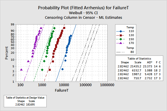
To see how well the model fits, you will draw a probability plot based on the standardized residuals.
1 Open the worksheet INSULATE.MTW.
2 Choose Stat > Reliability/Survival > Accelerated Life Testing.
3 In Variables/Start variables, enter FailureT. In Accelerating variable, enter Temp.
4 From Relationship, choose Arrhenius.
5 Click Censor. In Use censoring columns, enter Censor, then click OK.
6 Click Graphs. In Design value to include on plot, enter 80. Click OK.
7 Click Estimate. In Enter new predictor values, enter Design, then click OK in each dialog box.
Session window output
Accelerated Life Testing: FailureT versus Temp
Response Variable: FailureT
Censoring Information Count Uncensored value 66 Right censored value 14
Censoring value: Censor = C
Estimation Method: Maximum Likelihood
Distribution: Weibull
Relationship with accelerating variable(s): Arrhenius
Regression Table
Standard 95.0% Normal CI Predictor Coef Error Z P Lower Upper Intercept -15.1874 0.986180 -15.40 0.000 -17.1203 -13.2546 Temp 0.830722 0.0350418 23.71 0.000 0.762042 0.899403 Shape 2.82462 0.256969 2.36332 3.37596
Log-Likelihood = -564.693
Table of Percentiles
Standard 95.0% Normal CI Percent Temp Percentile Error Lower Upper 50 80 159584 27446.9 113918 223557 50 100 36948.6 4216.51 29543.4 46209.9 |
Graph window output:


From the Regression Table, you get the coefficients for the regression model. For a Weibull distribution, this model describes the relationship between temperature and failure time for the insulation:
Loge (failure time) = -15.1874 + 0.83072 (ArrTemp) + 1/2.8246 ep
where ep = the pth percentile of the standard extreme value distribution
|
ArrTemp = |
11604.83 |
|
Temp + 273.16 |
The Table of Percentiles displays the 50th percentiles for the temperatures
that you entered. The 50th percentile is a good estimate of how long the
insulation will last in the field. At 80
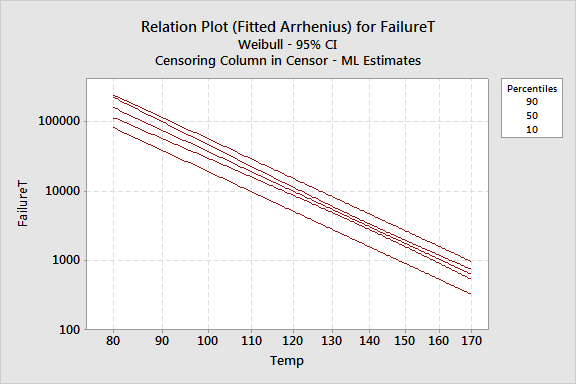
With the relation plot, you can look at the distribution of failure times for each temperature - in this case, the 10th, 50th, and 90th percentiles.
The probability plot based on the fitted model can help you determine whether the distribution, transformation, and assumption of equal shape (Weibull) at each level of the accelerating variable are appropriate. In this case, the points fit the lines adequately, thereby verifying that the assumptions of the model are appropriate for the accelerating variable levels.