main topic interpreting results session command see also
Suppose you work for a light bulb manufacturer and have been asked to determine bulb life for two types of bulbs at typical household voltages. The typical line voltage entering a house is 117 volts + 10% (or 105 to 129 volts).
You subject the two bulbs to five stress levels within that range: 108, 114, 120, 126, and 132 volts, and define an event as: The bulb fails before 800 hours.
1 Open the worksheet LIGHTBUL.MTW.
2 Choose Stat > Reliability/Survival > Probit Analysis.
3 Choose Response in event/trial format.
4 In Number of events, enter Blows. In Number of trials, enter Trials.
5 In Stress (stimulus), enter Volts.
6 In Factor (optional), enter Type.
7 From Assumed distribution, choose Weibull.
8 Click Estimate. In Estimate probabilities for these stress values, enter 117, then click OK.
9 Click Graphs. Uncheck Display confidence intervals on above plots. Click OK in each dialog box.
Session Window Output:
Probit Analysis: Blows, Trials versus Volts, Type
Distribution: Weibull
Response Information
Variable Value Count Blows Event 192 Non-event 308 Trials Total 500
Factor Information
Factor Levels Values Type 2 A, B
Estimation Method: Maximum Likelihood
Regression Table
Standard Variable Coef Error Z P Constant -97.0190 7.67326 -12.64 0.000 Volts 20.0192 1.58695 12.61 0.000 Type B 0.179368 0.159832 1.12 0.262 Natural Response 0
Test for equal slopes: Chi-Square = 0.258463 DF = 1 P-Value = 0.611
Log-Likelihood = -214.213
Goodness-of-Fit Tests
Method Chi-Square DF P Pearson 2.51617 7 0.926 Deviance 2.49188 7 0.928
Type = A
Tolerance Distribution
Parameter Estimates
Standard 95.0% Normal CI Parameter Estimate Error Lower Upper Shape 20.0192 1.58695 17.1384 23.3842 Scale 127.269 0.737413 125.832 128.722
Table of Percentiles
95.0% Fiducial Standard CI Percent Percentile Error Lower Upper 1 101.141 1.84244 96.9868 104.341 2 104.731 1.63546 101.043 107.573 3 106.901 1.50897 103.501 109.527 4 108.476 1.41713 105.287 110.946 5 109.720 1.34490 106.698 112.068 6 110.753 1.28539 107.868 113.001 7 111.639 1.23483 108.872 113.802 8 112.416 1.19095 109.752 114.506 9 113.110 1.15225 110.536 115.135 10 113.737 1.11771 111.246 115.706 20 118.082 0.898619 116.121 119.700 30 120.881 0.790097 119.201 122.342 40 123.069 0.735850 121.550 124.472 50 124.960 0.717911 123.523 126.372 60 126.714 0.728520 125.299 128.191 70 128.454 0.764984 127.010 130.050 80 130.330 0.830361 128.802 132.108 90 132.683 0.943441 130.989 134.754 91 132.980 0.959732 131.261 135.092 92 133.298 0.977596 131.551 135.455 93 133.641 0.997402 131.864 135.848 94 134.018 1.01968 132.206 136.280 95 134.439 1.04522 132.587 136.765 96 134.922 1.07534 133.023 137.323 97 135.500 1.11242 133.542 137.993 98 136.243 1.16159 134.207 138.857 99 137.358 1.23831 135.198 140.159
Table of Survival Probabilities
95.0% Fiducial CI Stress Probability Lower Upper 117 0.830608 0.780679 0.878549
Type = B
Tolerance Distribution
Parameter Estimates
Standard 95.0% Normal CI Parameter Estimate Error Lower Upper Shape 20.0192 1.58695 17.1384 23.3842 Scale 126.134 0.704348 124.761 127.522
Table of Percentiles
95.0% Fiducial Standard CI Percent Percentile Error Lower Upper 1 100.239 1.86171 96.0399 103.471 2 103.797 1.65621 100.059 106.673 3 105.947 1.53027 102.496 108.607 4 107.508 1.43857 104.267 110.012 5 108.742 1.36626 105.666 111.123 6 109.765 1.30652 106.828 112.045 7 110.643 1.25563 107.823 112.837 8 111.413 1.21135 108.697 113.533 9 112.101 1.17218 109.476 114.156 10 112.723 1.13711 110.180 114.720 20 117.028 0.910842 115.029 118.659 30 119.803 0.792908 118.102 121.256 40 121.972 0.727988 120.452 123.344 50 123.845 0.698947 122.429 125.203 60 125.584 0.698766 124.211 126.984 70 127.309 0.725223 125.925 128.806 80 129.168 0.781440 127.719 130.828 90 131.500 0.885656 129.901 133.434 91 131.794 0.901010 130.172 133.767 92 132.109 0.917912 130.461 134.125 93 132.449 0.936720 130.773 134.513 94 132.822 0.957949 131.114 134.939 95 133.240 0.982380 131.493 135.418 96 133.719 1.01129 131.927 135.969 97 134.292 1.04700 132.444 136.631 98 135.028 1.09453 133.104 137.484 99 136.132 1.16901 134.090 138.772
Table of Survival Probabilities
95.0% Fiducial CI Stress Probability Lower Upper 117 0.800867 0.745980 0.854567
Table of Relative Potency Factor: Type
Relative 95.0% Fiducial CI Comparison Potency Lower Upper A VS B 0.991080 0.975363 1.00678 |
Graph window output:

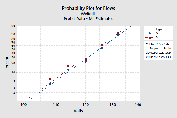
The goodness-of-fit tests (p-values = 0.926, 0.928) and the probability plot suggest that the Weibull distribution fits the data adequately. Since the test for equal slopes is not significant (p-value = .611), the comparison of light bulbs will be similar regardless of the voltage level. In this case, the light bulbs A and B are not significantly different because the coefficient associated with type B is not significantly different than 0 (p-value = .262).
At 117 volts, what percentage of the bulbs lasts beyond 800 hours? Eight-three percent of the bulb A's and 80% of the bulb B's last beyond 800 hours.
At what voltage do 50% of the bulbs fail before 800 hours? The table of percentiles shows you that 50% of bulb A's fail before 800 hours at 124.96 volts; 50% of bulb B's fail before 800 hours at 123.85 volts.