main topic interpreting results session command see also
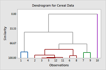
You make measurements on five nutritional characteristics (protein, carbohydrate, and fat content, calories, and percent of the daily allowance of Vitamin A) of 12 breakfast cereal brands. The example and data are from p. 623 of [6]. The goal is to group cereal brands with similar characteristics. You use clustering of observations with the complete linkage method, squared Euclidean distance, and you choose standardization because the variables have different units. You also request a dendrogram and assign different line types and colors to each cluster.
1 Open the worksheet CEREAL.MTW.
2 Choose Stat > Multivariate > Cluster Observations.
3 In Variables or distance matrix, enter Protein-VitaminA.
4 From Linkage Method, choose Complete and from Distance Measure choose Squared Euclidean.
5 Check Standardize variables.
6 Under Specify Final Partition by, choose Number of clusters and enter 4.
7 Check Show dendrogram.
8 Click Customize. In Title, enter Dendrogram for Cereal Data.
9 Click OK in each dialog box.
Session window output
Cluster Analysis of Observations: Protein, Carbo, Fat, Calories, VitaminA
Standardized Variables, Squared Euclidean Distance, Complete Linkage Amalgamation Steps
Number of obs. Number of Similarity Distance Clusters New in new Step clusters level level joined cluster cluster 1 11 100.000 0.0000 5 12 5 2 2 10 99.822 0.0640 3 5 3 3 3 9 98.792 0.4347 3 11 3 4 4 8 94.684 1.9131 6 8 6 2 5 7 93.406 2.3730 2 3 2 5 6 6 87.329 4.5597 7 9 7 2 7 5 86.189 4.9701 1 4 1 2 8 4 80.601 6.9810 2 6 2 7 9 3 68.079 11.4873 2 7 2 9 10 2 41.409 21.0850 1 2 1 11 11 1 0.000 35.9870 1 10 1 12
Final Partition Number of clusters: 4
Average Maximum Within distance distance Number of cluster sum from from observations of squares centroid centroid Cluster1 2 2.48505 1.11469 1.11469 Cluster2 7 8.99868 1.04259 1.76922 Cluster3 2 2.27987 1.06768 1.06768 Cluster4 1 0.00000 0.00000 0.00000
Cluster Centroids
Variable Cluster1 Cluster2 Cluster3 Cluster4 Grand centroid Protein 1.92825 -0.333458 -0.20297 -1.11636 0.0000000 Carbo -0.75867 0.541908 0.12645 -2.52890 0.0000000 Fat 0.33850 -0.096715 0.33850 -0.67700 0.0000000 Calories 0.28031 0.280306 0.28031 -3.08337 -0.0000000 VitaminA -0.63971 -0.255883 2.04707 -1.02353 -0.0000000
Distances Between Cluster Centroids
Cluster1 Cluster2 Cluster3 Cluster4 Cluster1 0.00000 2.67275 3.54180 4.98961 Cluster2 2.67275 0.00000 2.38382 4.72050 Cluster3 3.54180 2.38382 0.00000 5.44603 Cluster4 4.98961 4.72050 5.44603 0.00000 |
Graph window output

Minitab displays the amalgamation steps in the Session window. At each step, two clusters are joined. The table shows which clusters were joined, the distance between them, the corresponding similarity level, the identification number of the new cluster (this number is always the smaller of the two numbers of the clusters joined), the number of observations in the new cluster, and the number of clusters. Amalgamation continues until there is just one cluster.
The amalgamation steps show that the similarity level decreases by increments of about 6 or less until it decreases by about 13 at the step from four clusters to three. This indicates that four clusters are reasonably sufficient for the final partition. If this grouping makes intuitive sense for the data, then it is probably a good choice.
When you specify the final partition, Minitab displays three additional tables. The first table summarizes each cluster by the number of observations, the within cluster sum of squares, the average distance from observation to the cluster centroid, and the maximum distance of observation to the cluster centroid. In general, a cluster with a small sum of squares is more compact than one with a large sum of squares. The centroid is the vector of variable means for the observations in that cluster and is used as a cluster midpoint. The second table displays the centroids for the individual clusters while the third table gives distances between cluster centroids.
The dendrogram displays the information in the amalgamation table in the form of a tree diagram. In our example, cereals 1 and 4 make up the first cluster; cereals 2, 3, 5, 12, 11, 6, and 8 make up the second; cereals 7 and 9 make up the third; cereal 10 makes up the fourth.