main topic interpreting results session command see also
A psychiatric center records these data for each patient:
1: Normal reason
2: Other reason; for example against medical advice, court-ordered, absent without leave, and so on
Reason for discharge is binary data because the values are either normal or other. Therefore, a binary logistic regression analysis is appropriate to investigate whether length of stay affects a patient's reason for discharge.
1 Open the worksheet HCC.MTW.
2 Choose Stat > Regression > Binary Fitted Line Plot.
3 In Response, enter Reason.
4 In Predictor, enter Length.
5 Click Options.
6 In Increment for odds ratio, enter 7.
7 Click OK.
8 Click Graphs.
9 Choose Three in one.
10 Click OK in each dialog box.
Session window output
|
Graph window output


The Session window output contains these parts:
Method: Displays the link function. In the output, you can see that the model uses the logit link function.
Response Information: Displays the number of events, nonevents, and the total. In the output, you can see that the data contain 42 normal discharges and 16 other discharges.
Deviance Table: Displays the likelihood ratio test p-values for the coefficients. In the output, you can see that the estimated coefficient for Length has a p-value that is greater than 0.05. With an a-level of 0.05, the evidence is not sufficient to show that the coefficient is not zero.
Model Summary: Displays the deviance R2, adjusted deviance R2, and Akaike Information Criterion (AIC). Use these statistics to compare different models:
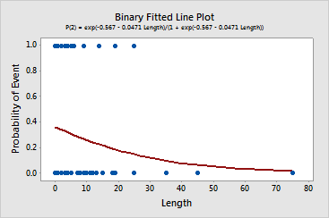
Coefficients: Displays the estimated coefficients, standard error of the coefficients and variance inflation factors (VIF). The estimated coefficient of -0.0471 for Length represents the change in the log of P(the hospital discharges a patient for other reasons)/P(the hospital discharges a patient for normal reasons) when the length of stay changes by one day.
Odds ratios for continuous predictors: Displays the unit of change, odds ratio, and a confidence interval for the odds ratio. The unit of change for Length in the analysis is 7 days. The odds ratio for time is estimated to be 0.7189, with a confidence interval from 0.4350 – 1.1881. Typical interpretation of the ratio is that if the length of stay increases by one week, the odds that the hospital discharges the patient for other reasons decrease by 0.7189 times.
Fits and Diagnostics for Unusual Observations: Displays statistics about observations with standardized residuals greater than 2 or large leverage values. The statistics are the observed probability, the predicted probability, the residual, and the standardized residual. Observation 32 is unusual because the length of stay, 45, is unusually long and still has enough weight on the regression to deserve attention. Observation 58 is unusual because the patient was discharged for other reasons, even though the model predicted that the hospital would discharge the patient for normal reasons if the patient stayed for as long as 25 days.
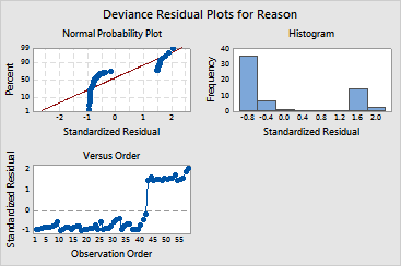
Plots: In the example, you chose three diagnostic plots. These plots do not reveal any points that deviate from the rest of the data, although you can see that observation 58 has the largest residual. Because other discharges are rare, the model predicts higher probabilities that the hospital discharged patients for normal reasons. When the hospital discharged a patient for other reasons, the residuals are farther from zero than when the hospital discharged a patient for normal reasons.
The residuals do not follow a normal distribution. Therefore, the confidence intervals on the binary fitted line plot are unreliable.
The binary fitted line plot shows that the relationship between length of stay and reason for discharge is weak.