main topic interpreting results session command see also
You are a researcher who is interested in understanding the effect of smoking and weight upon resting pulse rate. Because you have categorized the response-pulse rate-into low and high, a binary logistic regression analysis is appropriate to investigate the effects of smoking and weight upon pulse rate.
1 Open the worksheet EXH_REGR.MTW.
2 Choose Stat > Regression > Binary Logistic Regression > Fit Binary Logistic Model.
3 For the type of data, choose Response in binary response/frequency format.
4 In Response, enter RestingPulse.
5 In Response event, choose Low.
6 In Continuous predictors, enter Weight.
7 In Categorical predictors, enter Smokes.
8 Click Coding.
9 In Increment, enter 10.
10 Click OK.
11 Click Graphs.
12 Choose Three in one.
13 Click OK in each dialog box.
Session window output
|
Graph window output

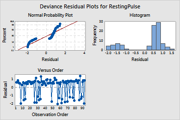
The Session window output contains ten parts. The graph window contains three plots in one graph.
Method: Displays the link function and other information about the analysis. This model uses the logit link function.
Response Information: Displays the number of missing observations and the number of observations that fall into each of the two response categories. The response value that has been designated as the reference event is the first entry under Value and is labeled as the event. In this case, the reference event is low pulse rate.
Deviance Table: Displays the likelihood ratio test p-values for the coefficients. In the output, you can see that the estimated coefficients for both Smokes (p = 0.030) and Weight (p = 0.031) have p-values that are less than 0.05. These results indicate that there is sufficient evidence that the coefficients are not zero using an a-level of 0.05. The p-value for the overall regression tests the null hypothesis that all the coefficients for predictors are equal to zero. The alternative hypothesis is that at least one of the coefficients for a predictor is not equal to zero. In this example, the p-value is 0.023. This p-value indicates that there is sufficient evidence that at least one of the coefficients is different from zero, given that your accepted a-level is greater than 0.023.
Model Summary: Displays the statistics you can use to compare how well different models fit the data. Higher values of deviance R2 and adjusted deviance R2 indicate a better fit. Smaller values of Akaike Information Criterion (AIC) indicate a better fit. The current model has a deviance R2 value of 7.48%, an adjusted R2 value of 5.51%, and an AIC of 99.64. Another model might have better fit statistics.
Coefficients: Shows the estimated coefficients, standard error of the coefficients, and variance inflation factors (VIF). When you use the logit link function, you also see the odds ratio and a 95% confidence interval for the odds ratio.
The estimated coefficient of -1.193 for Smokes represents the change in the log of P(low pulse)/P(high pulse). The interpretation of the coefficient is for when the subject smokes compared to when he/she does not smoke. The coefficient assumes that the covariate Weight is constant. The estimated coefficient for Weight is 0.0250. The coefficient represents the change in the log of P(low pulse)/P(high pulse) with a 1 unit (1 pound) increase in Weight, with the factor Smokes held constant.
Odds Ratios for Continuous Predictors: Although there is evidence that the estimated coefficient for Weight is not zero, the estimated coefficient is very close to zero (0.0250). This odds ratio indicates that a 1 pound increase in weight minimally affects a person's resting pulse rate. A more meaningful difference would be found if you compared subjects with a larger weight difference with the odds ratio. For example, if the weight unit is 10 pounds, the odds ratio becomes 1.2843. The larger odds ratio indicates that the odds of a subject having a low pulse increases by 1.2843 times with each 10 pound increase in weight.
Odds Ratios for Categorical Predictors: For Smokes, the negative coefficient of -1.193 and the odds ratio of 0.3033 indicate that subjects who smoke tend to have a higher resting pulse rate than subjects who do not smoke. Given that subjects have the same weight, the odds ratio can be interpreted as the odds of smokers in the sample having a low pulse being 30% of the odds of non-smokers having a low pulse.
Regression Equation: Displays the transformation that changes the linear equation into a predicted probability and a linear equation for each combination of categorical predictors. In this case, there are two equations, one for each level of the Smokes variable. The constant term is more negative for the people who smoke, so these people have a lower probability of having a lower resting pulse. Because there is no interaction with weight in the model, the coefficient is the same in both equations.
Goodness-of-Fit Tests: Displays Pearson, deviance, and Hosmer-Lemeshow goodness-of-fit tests. The goodness-of-fit tests, with p-values ranging from 0.348 to 0.724, indicate that there is insufficient evidence to claim that the model does not fit the data adequately. If the p-value is less than your accepted a-level, the test would reject the null hypothesis of an adequate fit.
Fits and Diagnostics for Unusual Observations: Displays observations that have large standardized residuals or large leverage values. In this case, observation 56 is not fit well by the model. You might further investigate this case to see why the model did not fit it well. Observation 86 can have large influence on the model. You might fit the model without this case to see how much influence the observation has on the results.
Plots: In the example, you chose three residual plots. The normal probability plot of the residuals is not a straight line, and the histogram of the residuals is bi-modal. You should be cautious about how you interpret output that relies on normal theory, like confidence intervals for the predicted probabilities.