main topic interpreting results session command see also
These data are the results of a survey given to an MBA class at the beginning of the semester. The data contain some characteristics about the students' education and finances and uses them to examine which credit cards students have.
1 Open the worksheet MBASURVEY.MTW.
2 Choose Stat > Regression > Binary Logistic Regression > Fit Binary Logistic Model.
3 In Response, enter AmEx. In Continuous predictors enter Cash AIncome. In Categorical predictors enter HDegree.
4 Click Model. In Predictors, highlight Cash. Next to Terms through order, click Add.
5 In Predictors, highlight Cash and AIncome. Next to Interactions through order, click Add. Click OK in each dialog box.
6 Choose Stat > Regression > Binary Logistic Regression > Fit Binary Logistic Model.
7 In Response, enter MC. In Continuous predictors enter GMAT Cash AIncome. In Categorical predictors enter Gender HDegree.
8 Click Model.
9 Click Default.
10 Click OK in each dialog box.
11 Choose Stat > Regression > Binary Logistic Regression > Response Optimizer.
9 Under Goal, choose Maximize for both AmEx and MC.
10 Click Setup.
11 Under Lower enter 0.9 for MC and 0.8 for AMEX.
12 Click OK in each dialog box.
Session Window Output
Binary Logistic Regression: AmEx versus Cash, AIncome, HDegree
Binary Logistic Regression: MC versus GMAT, Cash, AIncome, Gender, HDegree
Response Optimization: MC, AmEx
Parameters
Response Goal Lower Target Upper Weight Importance MC Maximum 0.9 1 1 1 AmEx Maximum 0.8 1 1 1
Solution
MC AmEx Fitted Fitted Composite Solution GMAT Cash AIncome Gender HDegree Probability Probability Desirability 1 44 349 114424 Male Masters 1.00000 1.00000 0.99999
Multiple Response Prediction
Variable Setting GMAT 44 Cash 349 AIncome 114424 Gender Male HDegree Masters
Fitted Response Probability SE Fit 95% CI MC 1.00000 0.00001 (0.06415, 1.00000) AmEx 1.00000 0.00000 (0.00053, 1.00000) |
Graph Window Output

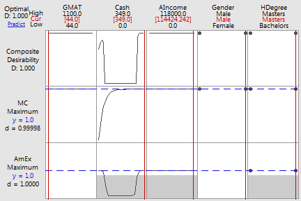
The combined or composite desirability of these two responses is about 1.
To obtain this desirability, you would set the factor levels at the values shown under Solution. That is, the student's Graduate Management Admissions Test (GMAT) score would be 44, the student would carry $349 in cash, the student's annual income would be $114,424, the student would be male, and the student has a master's degree. The confidence intervals indicate the precision of these predictions, which are very wide. While the predictions show a high probability, this model does not provide a high degree of confidence.
In this case, the high and low values of the GMAT scores call attention to a problem with the data. The student who reported an 1100 gave their Graduate Record Examination score instead of their GMAT score, and the student who reported a 44 gave the results for only a portion of the test. After the surveyor corrects the data, they can refit the models.
If you want to adjust the factor settings of this initial solution, you can use the plot. Move the vertical bars to change the factor settings and see how the individual desirability (d) of the responses and the composite desirability change.
Keep in mind that these results are based on model equations. You should be sure that your models are adequate before interpreting the plots.