Example of a surface plot for a binary regression model
main topic     interpreting results     session command     see also 

These data are the results of a survey given to an MBA class at the beginning of the semester. The data contain some characteristics about the students' education and finances and uses them to examine which credit cards students have.

1    Open the worksheet MBASURVEY.MTW.

2    Choose Stat > Regression > Binary Logistic Regression > Fit Binary Logistic Model

3    In Response, enter AmEx. In Continuous predictors enter Cash AIncome. In Categorical predictors enter HDegree.

4    Click Model. In Predictors, highlight Cash. Next to Terms through order, click Add.

5    In Predictors, highlight Cash and AIncome. Next to Interactions through order, click Add. Click OK in each dialog box.

6    Choose Stat > Regression > Binary Logistic Regression > Surface Plot.

7    Click Settings. In Hold categorical variables at, change Setting to Masters. Click OK in each dialog box.

Graph window output

Interpreting the results

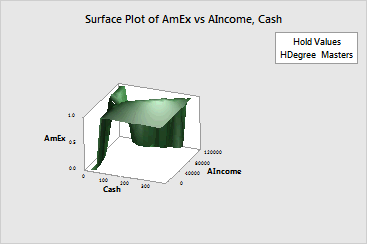
The surface peaks where cash is highest and annual income is lowest. The more cash a student carries and the lower their annual income, the more likely that the student carries an American Express card. For this data, no values are near cash values of 400 and annual income values of 0. The region where the surface plot is flat is where extrapolation occurs.

The predictions are only for students whose highest level of education is a master's degree. To look at the model for students with other highest levels of education, change the hold value in Settings.

Keep in mind that this plot is based on a model equation. You should be sure that your model is adequate before interpreting the plots.