main topic interpreting results session command see also
You are studying the relationship between a particular machine setting and the amount of energy consumed. This relationship is known to have considerable curvature, and you believe that a log transformation of the response variable will produce a more symmetric error distribution. You choose to model the relationship between the machine setting and the amount of energy consumed with a quadratic model.
1 Open the worksheet EXH_REGR.MTW.
2 Choose Stat > Regression > Fitted Line Plot.
3 In Response (Y), enter EnergyConsumption.
4 In Predictor (X), enter MachineSetting.
5 Under Type of Regression Model, choose Quadratic.
6 Click Options. Under Transformations, check Logten of Y and Display logscale for Y variable. Under Display Options, check Display confidence interval and Display prediction interval. Click OK in each dialog box.
Session window output
Polynomial Regression Analysis: EnergyConsumption versus MachineSetting
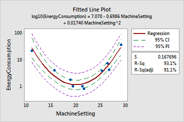
The regression equation is log10(EnergyConsumption) = 7.070 - 0.6986 MachineSetting + 0.01740 MachineSetting^2
S = 0.167696 R-Sq = 93.1% R-Sq(adj) = 91.1%
Analysis of Variance
Source DF SS MS F P Regression 2 2.65326 1.32663 47.17 0.000 Error 7 0.19685 0.02812 Total 9 2.85012
Sequential Analysis of Variance
Source DF SS F P Linear 1 0.03688 0.10 0.754 Quadratic 1 2.61638 93.04 0.000
Fitted Line: EnergyConsumption versus MachineSetting |
Graph window output

The quadratic model (p-value
= 0.000, or actually p-value < 0.0005) appears to provide a good fit
to the data. The R![]() indicates that machine setting accounts for 93.1% of the variation in
log10 of the energy consumed. A visual
inspection of the plot reveals that the data are randomly spread about
the regression line,
implying no systematic lack-of-fit. The 95% confidence limits
(95% CI) for the log10 of energy
consumed and the 95% prediction limits
(95% PI) for new observations are also shown.
indicates that machine setting accounts for 93.1% of the variation in
log10 of the energy consumed. A visual
inspection of the plot reveals that the data are randomly spread about
the regression line,
implying no systematic lack-of-fit. The 95% confidence limits
(95% CI) for the log10 of energy
consumed and the 95% prediction limits
(95% PI) for new observations are also shown.