Example of nonlinear regression
main topic     interpreting results     session command     see also 

Researchers for the National Institute of Standards and Technology (NIST) want to understand the relationship between semiconductor electron mobility and the natural log of the density. The data are publicly available from the NIST (Thurber, R., 1979). Prior research suggests that a nonlinear rational model (the ratio of 2 polynomials) with 7 parameters provides an adequate fit. The methods discussed in [4] yield the starting values.

1    Open the worksheet MOBILITY.MTW.

2    Choose Stat > Regression > Nonlinear Regression.

3    In Response, enter Mobility.

4    In Expectation Function, under Edit directly, enter (b1+b2*'Density Ln'+b3*'Density Ln'**2+b4*'Density Ln'**3)/  (1+b5*'Density Ln'+b6*'Density Ln'**2+b7*'Density Ln'**3).

5    Click Parameters.

6    Under Required starting values, in order from b1 to b7, enter one value per cell: 1300, 1500, 500, 75, 1, 0.4, 0.05.

7    Click OK.

8    Click Graphs.

9    Under Plot of fitted curve with data, check Display confidence interval and Display prediction interval.

10  Under Residuals, choose Four in one.

11  Click OK.

12  Click Results.

13  Check Display confidence intervals.

14  Click OK in each dialog box.

Session Window output

Graph window output

Interpreting the results

Session window output

Minitab achieved the convergence criteria in 27 iterations using the Gauss-Newton algorithm with the expectation function and parameter starting values that you specified. However, convergence, by itself, does not guarantee an optimal model fit or a minimized sum of squared errors (SSE). Convergence on incorrect parameter values can occur due to a local SSE minimum, bad starting values, or an incorrect expectation function. Therefore, it is crucial to examine the parameter values, fitted line plot, and residual plots to ensure that the model adequately fits the data and that the algorithm converged on the global SSE minimum.

The convergence yields the following equation:

Mobility = (1288.14 + 1491.08 * 'Density Ln' + 583.238 * 'Density Ln' ** 2 + 75.4167 * 'Density Ln' ** 3) / 

(1 + 0.966295 * 'Density Ln' + 0.397973 * 'Density Ln' ** 2 + 0.0497273 * 'Density Ln' ** 3)

Minitab does not calculate p-values for the parameters. For linear regression, the null hypothesis value for every parameter is 0, for no effect, and the p-value is based on this value. In nonlinear regression, the correct null hypothesis value for each parameter depends on the expectation function and the parameter's place in it. Instead of the p-value, Minitab can display a confidence interval for each parameter estimate. Use your knowledge of the subject area and expectation function to determine if this range is reasonable and if it indicates a significant effect.

For example, the point estimate for parameter b1 is 1288.14 and the 95% confidence interval is (1278.61, 1297.67). The researchers consider this to be a reasonable range that implies significance.  

For some data sets, expectation functions, and confidence levels, one or both confidence bounds may not exist. For the mobility data, parameters b5 and b6 do not have an upper bound. When a confidence interval has a missing bound, a lower confidence level might produce a two-sided interval. In this case, if you reduce the confidence level to 92%, Minitab can calculate two-sided intervals for b5 and b6.

For this data set, Minitab does not perform the Lack of Fit test because there are no replicates. Look at the model summary values, fitted line plot, and residual plots to assess fit.

For nonlinear regression, Minitab does not calculate the R2  or p-value for the overall model because these values are generally meaningless outside of the linear model context. Therefore, when researchers assess the fit and compare competing nonlinear models,  they often choose between them based on subject area knowledge, the one with the smallest Final SSE or S value, and the graphical output.

The S value is generally more intuitive to interpret, both by itself and in comparison to competing values, because S is expressed in the same units as the response variable (electron mobility). In this case, S is 13.7146 which indicates that the observed electron mobility values fall a standard distance (roughly an average absolute distance) of 13.7146 units from the fitted mobility values.

The warning about highly correlated parameters indicates that at least one pair of parameters has a correlation greater than an absolute value of 0.99. You can consider whether to implement the warning's recommendations.

Graph window output

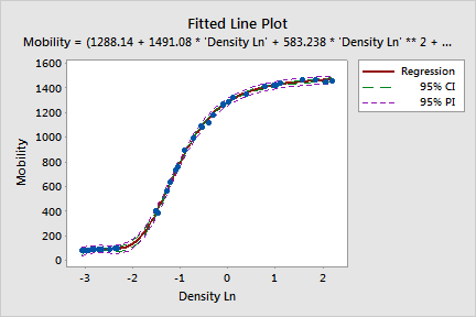
The fitted line plot with the raw data appears to show a reasonable fit. The points are fairly close to the line and follow the curve without any systematic departures from it. Because the equation is so long, it does not display properly on the graph. You can edit the graph or look in the Session Window output to view the full equation.

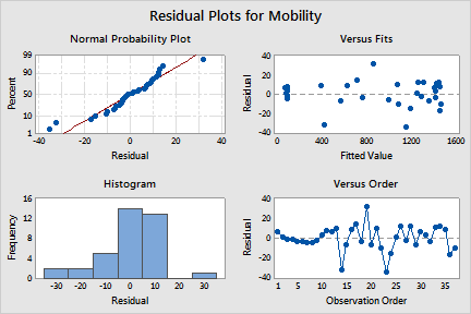
The histogram does not show any outliers, but it is somewhat skewed. However, use the normal probability plot to assess normality.

The normal probability plot shows an approximately linear pattern consistent with a normal distribution.

The plot of residuals versus the fitted values shows a random pattern, which suggests that the residuals have constant variance. See [9] for information on non-constant variance.

The residuals versus order plot shows the order that the data was collected and can be used to find non-random error, especially of time-related effects. The residuals versus order plot displays a non-random pattern for the first 13 data points. You should investigate these points to determine why this pattern exists and determine if there is something wrong with the measurement system or with your data collection procedures.