You are a wine producer who wants to know how the chemical composition
of your wine relates to sensory evaluations. You have 37 Pinot Noir wine
samples, each described by 17 elemental concentrations (Cd, Mo, Mn, Ni,
Cu, Al, Ba, Cr, Sr, Pb, B, Mg, Si, Na, Ca, P, K) and a score on the wine's
aroma from a panel of judges. You want to predict the aroma score from
the 17 elements and determine that PLS is an appropriate technique because
the ratio of samples to predictors is low. Data are from [12].
You want to include all elements (Cd-K) and all two-way interactions that
include Cd in the model.
1 Open the worksheet WINEAROMA.MTW.
2 Choose Stat
> Regression > Partial Least Squares.
3 In Responses,
enter Aroma.
4 In Model,
enter Cd-K Cd*Mo Cd*Mn Cd*Ni Cd*Cu Cd*Al
Cd*Ba Cd*Cr Cd*Sr Cd*Pb Cd*B Cd*Mg Cd*Si Cd*Na Cd*Ca Cd*P Cd*K.
5 Click Options.
6 Under Cross-Validation, choose
Leave-one-out.
Click OK.
7 Click
Graphs,
then check Model
selection plot,
Response plot,
Std Coefficient plot, Distance plot, Residual versus leverage,
and Loading plot.
Uncheck Coefficient plot.
8 Click
OK in each dialog
box.
Session window output
|
PLS Regression: Aroma versus Cd, Mo, Mn, Ni, Cu, Al, Ba, Cr, Sr, Pb, B, Mg, Si, Na, Ca, P, K
Method
Cross-validation Leave-one-out
Components to evaluate Set
Number of components evaluated 10
Number of components selected 4
Analysis of Variance for Aroma
Source DF SS MS F P
Regression 4 34.5514 8.63784 41.55 0.000
Residual Error 32 6.6519 0.20787
Total 36 41.2032
Model Selection and Validation for Aroma
Components X Variance Error R-Sq PRESS R-Sq (pred)
1 0.158849 14.9389 0.637435 23.3439 0.433444
2 0.442267 12.2966 0.701564 21.0936 0.488060
3 0.522977 7.9761 0.806420 19.6136 0.523978
4 0.594546 6.6519 0.838559 18.1683 0.559056
5 5.8530 0.857948 19.2675 0.532379
6 5.0123 0.878352 22.3739 0.456988
7 4.3109 0.895374 24.0041 0.417421
8 4.0866 0.900818 24.7736 0.398747
9 3.5886 0.912904 24.9090 0.395460
10 3.2750 0.920516 24.8293 0.397395
|
Graph window output


Interpreting the results
Session window output
· The
Method table indicates the number of components Minitab evaluated and
the number of components selected as the optimal model. The optimal model
is defined as the model with the highest predicted R2.
Minitab selected the four-component model as the optimal model, with a
predicted R2
of 0.56.
· Minitab
displays one Analysis of Variance table
per response based on the optimal model. The p-value
for aroma is 0.000, which is less than an alpha
of 0.05, providing sufficient evidence that the four-component model is
significant.
· Use
the Model Selection and Validation table to select the optimal number
of components for your model. Depending on your data or field of study,
you may determine that a model other than the one selected by cross-validation
is more appropriate. The model with four components, which was selected
by cross-validation, has an R2
of 83.8% and a predicted R2
of 55.9%.
· The
X-variance
indicates the amount of variance in the predictors that is explained by
the model. In this example, the four-component model explains 59.4% of
the variance in the predictors.
Graph window output
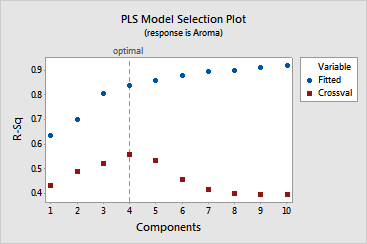
· The
model selection plot is a graphical display of the Model Selection and
Validation table. The vertical line indicates that the optimal model has
four components. You can see that the predictive ability of all models
with more than four components decreases significantly.
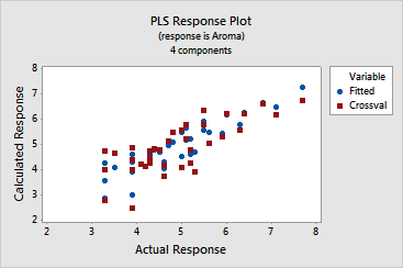
· The
response plot indicates that the model fits the data adequately because
the points are in a linear pattern, from the bottom left-hand corner to
the top right-hand corner. Although there are differences between the
fitted
and cross-validated fitted responses,
none are severe enough to indicate an extreme leverage
point.
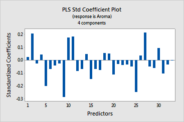
· The
coefficient plot displays the standardized coefficients
for the predictors. You can use this plot to interpret the magnitude and
sign of the coefficients. The elements Mo, Cu, Sr, Pb, B, Ca, Cd*Sr, Cd*B
have the largest standardized coefficients and the biggest impact on aroma.
The elements Mo, Pb, B, and Cd*B are positively related to aroma, while
Cu, Sr, Ca, and Cd*Sr are negatively related.
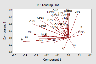
· The
loading plot compares the relative influence of the predictors on the
response. In this example, Cu and Ni have very short lines, indicating
that they have low x-loadings
and are not related to aroma. The elements Sr, Mg, and Ba have long lines,
indicating that they have higher loadings and are more related to aroma.
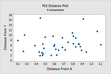
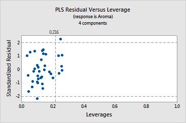
· The distance
plot and the residual versus leverage plot display outliers
and leverages. By brushing the distance plot, you can see that compared
to the rest of the data:
-
observations
14 and 32 have a greater distance value on the y-axis
-
observations
in rows 1 and 37 have greater distance value on the x-axis
The residual versus leverage plot shows that:
-
observation
3 is an outlier because it is outside the horizontal reference lines
-
observations
5, 12, 14, 23, and 37 have extreme leverage values because they are to
the right of the vertical reference line
