A manufacturer produces molded resin parts. Contamination in hoses and
abrasions to resin pellets can lead to discolored streaks in the final
product. Higher temperatures and faster rates of transfer can cause pellets
to clump together. Clumps can be difficult to move through hoses and into
molds. The company collects data on the number of defects per hour.
1 Open
the worksheet ResinDefects.MTW.
2 Choose
Stat > Regression > Poisson Regression
> Fit Poisson Model.
3 In
Response enter
Discoloration Defects.
4 In
Continuous Predictors
enter Hours Since Cleanse and
Temperature.
5 In
Categorical Predictors
enter Size of Screw.
6 Click
Graphs.
7 In
Residuals for Plots,
choose Standardized.
8 Under
Residual Plots,
choose Four in One.
9 Click
OK in each dialog
box.
Session window output
|
Poisson Regression Analysis: Discoloratio versus Hours Since , Temperature, Size of Scre
Method
Link function Natural log
Categorical predictor coding (1, 0)
Rows used 36
Deviance Table
Source DF Adj Dev Adj Mean Chi-Square P-Value
Regression 3 56.670 18.8900 56.67 0.000
Hours Since Cleanse 1 4.744 4.7444 4.74 0.029
Temperature 1 38.800 38.8000 38.80 0.000
Size of Screw 1 13.126 13.1256 13.13 0.000
Error 32 31.607 0.9877
Total 35 88.277
Model Summary
Deviance Deviance
R-Sq R-Sq(adj) AIC
64.20% 60.80% 253.29
Coefficients
Term Coef SE Coef VIF
Constant 4.3982 0.0628
Hours Since Cleanse 0.01798 0.00826 1.00
Temperature -0.001974 0.000318 1.00
Size of Screw
small -0.1546 0.0427 1.00
Regression Equation
Discoloration Defects = exp(Y')
Size of
Screw
large Y' = 4.398 + 0.01798 Hours Since Cleanse - 0.001974 Temperature
small Y' = 4.244 + 0.01798 Hours Since Cleanse - 0.001974 Temperature
Goodness-of-Fit Tests
Test DF Estimate Mean Chi-Square P-Value
Deviance 32 31.60722 0.98773 31.61 0.486
Pearson 32 31.26713 0.97710 31.27 0.503
Fits and Diagnostics for Unusual Observations
Discoloration
Obs Defects Fit Resid Std Resid
33 43.00 58.18 -2.09 -2.18 R
R Large residual
|
|
|

Interpreting the results
Session window output
· The
p-value
for the regression model in the Analysis of Deviance table (0.000) shows
that the model estimated by the regression procedure is significant
at an a-level
of 0.05. This indicates that at least one coefficient is different from
zero.
· The
deviance R2
value indicates that the predictors explain 64.20% of the variance in
the number of discolorations. The adjusted deviance R2
is 60.80%,
which accounts for the number of predictors in the model. Use these values
to compare this model to other models.
· The
Akaike Information Criterion (AIC) value is 253.29. Use the AIC to compare
different models. The smaller the AIC, the better.
· The
coefficient for Hours Since Cleanse is 0.01798. Because the model uses
the natural log link function and the coefficient is small, the coefficient
indicates that the number of discolorations increases by about 1.8% each
hour. See Interpreting
the parameter estimates for more details.
· One
observation has a standardized residual less than -2. This point is not
fit well by the model. Because the residuals show that the model is inadequate,
you cannot evaluate whether the points are unusual yet.
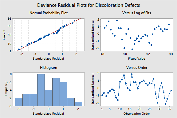
Graph window output
· The
normal probability plot
shows an approximately linear pattern consistent with a normal
distribution.
To investigate individual points, brush
the graph.
· The
plot of the residuals versus the fitted values
shows a distinct curve. This pattern indicates the model is inadequate.
For these data, the pattern is because the size of the screw and the temperature
interact but the interaction term is not in the model. The results are
not reliable until you add the interaction term and the residual plots
are satisfactory.
· On
the histogram,
no residuals look unusual. Three residuals are in bins that include -2
and 2. You
can verify that one of the residuals is less than -2 on the other residual
plots.
· The
plot of the residuals
versus order begins with 9 negative residuals. The middle portion of the
residuals tends to be higher than the residuals at the beginning and end
of the data set. For these data, the pattern is also because of the missing
interaction. The missing interaction looks like a time effect because
the data were not collected in a random order.
See Checking
your model and Identifying
outliers for more information about residual plots.
