Example of multiple regression
main topic     interpreting results     session command     see also 

As part of a test of solar energy, you measure the total heat flux from homes. You wish to examine whether total heat flux (HeatFlux) can be predicted by the position of the focal points in the east, south, and north directions. Data are from [33]. You found, using best subsets regression, that the best two-predictor model included the variables North and South and the best three-predictor added the variable East. You evaluate the three-predictor model using multiple regression.

1    Open the worksheet EXH_REGR.MTW.

2    Choose Stat > Regression > Regression > Fit Regression Model.

3    In Responses, enter HeatFlux.

4    In Continuous predictors, enter East South North.

5    Click Graphs.

6    Under Residuals for Plots, choose Standardized.

7    Under Residual Plots, choose Individual Plots. Check Histogram of residuals, Normal probability plot of the residuals, and Residuals versus fits.

8    Click OK in each dialog box.

Session window output

Interpreting the results

Session window output

·    The p-value for the regression model in the Analysis of Variance table (0.000) shows that the model estimated by the regression procedure is significant at an a-level of 0.05. This indicates that at least one coefficient is different from zero.

·    The p-values for the estimated coefficients of North and South are both 0.000, indicating that they are significantly related to HeatFlux. The p-value for East is 0.092, indicating that it is not related to HeatFlux at an a-level of 0.05. Additionally, the sequential sum of squares indicates that the predictor East doesn't explain a substantial amount of unique variance. This suggests that a model with only North and South may be more appropriate.  

·    The VIFs are all close to 1, which indicates that the predictors are not correlated. VIF values greater than 5-10 suggest that the regression coefficients are poorly estimated due to severe multicollinearity.

·    The R2 value indicates that the predictors explain 87.41% of the variance in HeatFlux. The adjusted R2  is 85.90%, which accounts for the number of predictors in the model. Both values indicate that the model fits the data well.

·    The predicted R2 value is 78.96%. Because the predicted R2 value is close to the R2  and adjusted R2 values, the model does not appear to be overfit and has adequate predictive ability.

·    Observations 4 and 22 are identified as unusual because the absolute value of the standardized residuals are greater than 2. This may indicate they are outliers. See Checking your model,  Identifying outliers, and Choosing a residual type.

Graph window output

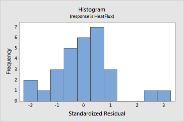
·    The histogram indicates that outliers may exist in the data, shown by the two bars on the far right side of the plot.

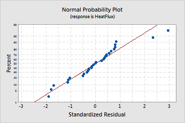
·    The normal probability plot shows an approximately linear pattern consistent with a normal distribution. The two points in the upper-right corner of the plot may be outliers. Brushing the graph identifies these points as 4 and 22, the same points that are labeled unusual observations in the output. See Checking your model and Identifying outliers.

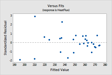
·    The plot of residuals versus the fitted values shows that the residuals get smaller (closer to the reference line) as the fitted values increase, which may indicate the residuals have non-constant variance. See [9] for information on non-constant variance.