main topic interpreting results session command see also
In the example of fitting an ARIMA model, you found that an AR(1) model with a twelfth seasonal difference gave a good fit to the food sector employment data. You now use this fit to predict employment for the next 12 months.
Step 1: Refit the ARIMA model without displaying the acf and pacf of the residuals
1 Perform steps 1- 4 of Example of ARIMA.
Step 2: Display a time series plot
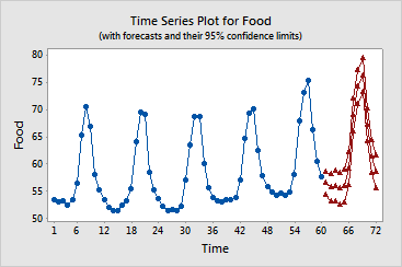
1 Click Graphs. Check Time series plot. Click OK.
Step 3: Generate the forecasts
1 Click Forecast. In Lead, enter 12. Click OK in each dialog box.
Session window output
ARIMA Model: Food
Estimates at each iteration
Iteration SSE Parameters 0 95.2343 0.100 0.847 1 77.5568 0.250 0.702 2 64.5317 0.400 0.556 3 56.1578 0.550 0.410 4 52.4345 0.700 0.261 5 52.2226 0.733 0.216 6 52.2100 0.741 0.203 7 52.2092 0.743 0.201 8 52.2092 0.743 0.200 9 52.2092 0.743 0.200
Relative change in each estimate less than 0.0010
Final Estimates of Parameters
Type Coef SE Coef T P AR 1 0.7434 0.1001 7.42 0.000 Constant 0.1996 0.1520 1.31 0.196
Differencing: 0 regular, 1 seasonal of order 12 Number of observations: Original series 60, after differencing 48 Residuals: SS = 51.0364 (backforecasts excluded) MS = 1.1095 DF = 46
Modified Box-Pierce (Ljung-Box) Chi-Square statistic
Lag 12 24 36 48 Chi-Square 11.3 19.1 27.7 * DF 10 22 34 * P-Value 0.338 0.641 0.768 *
Forecasts from period 60
95% Limits Period Forecast Lower Upper Actual 61 56.4121 54.3472 58.4770 62 55.5981 53.0251 58.1711 63 55.8390 53.0243 58.6537 64 55.4207 52.4809 58.3605 65 55.8328 52.8261 58.8394 66 59.0674 56.0244 62.1104 67 69.0188 65.9559 72.0817 68 74.1827 71.1089 77.2565 69 76.3558 73.2760 79.4357 70 67.2359 64.1527 70.3191 71 61.3210 58.2360 64.4060 72 58.5100 55.4240 61.5960 |
Graph window output

ARIMA gives forecasts, with 95% confidence limits, using the AR(1) model in both the Session window and a Graph window. The seasonality dominates the forecast profile for the next 12 months with the forecast values being slightly higher than for the previous 12 months.
| Minitab help | Stat | Graph | SixSigma | DOE | Glossary | Reliability | SPC,MSA,CPK | ||
|
|||||||||