main topic interpreting results session command see also
You wish to predict employment in a food preparation industry using past employment data. You want to use ARIMA to do this but first you use autocorrelation in order to help identify a likely model. Because the data exhibit a strong 12 month seasonal component, you take a difference at lag 12 in order to induce stationarity and look at the autocorrelation of the differenced series. There may be some long-term trend in these data, but the magnitude of it appears to be small compared to the seasonal component. If the trend was larger, you might consider taking another difference at lag 1 to induce stationarity.
1 Open the worksheet EMPLOY.MTW.
2 Choose Stat > Time Series > Differences.
3 In Series, enter Food.
4 In Store differences in, enter Food2.
5 In Lag, enter 12. Click OK.
6 Choose Stat > Time Series > Autocorrelation.
7 In Series, enter Food2. Click OK.
Session window output
Autocorrelation Function: Food2
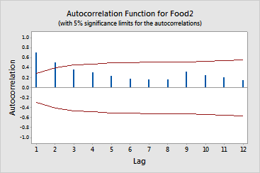
Lag ACF T LBQ 1 0.701388 4.86 25.12 2 0.512266 2.52 38.81 3 0.366882 1.60 45.99 4 0.310364 1.29 51.24 5 0.234743 0.94 54.32 6 0.173069 0.68 56.03 7 0.162046 0.63 57.57 8 0.170051 0.66 59.30 9 0.322438 1.24 65.70 10 0.252774 0.94 69.74 11 0.208020 0.76 72.54 12 0.150936 0.55 74.06
Autocorrelation for Food2 |
Graph window output

In the Session window, Minitab displays the autocorrelations, associated t-statistics, and Ljung-Box Q statistics. Because you did not specify the lag length, autocorrelation uses the default length of n / 4 for a series with less than or equal to 240 observations. Minitab generates an autocorrelation function (ACF) with approximate a = 0.05 critical bands for the hypothesis that the correlations are equal to zero.
The ACF for these data shows large positive, significant spikes at lags 1 and 2 with subsequent positive autocorrelations that do not die off quickly. This pattern is typical of an autoregressive process.
See Example of Testing Autocorrelations to test the null hypothesis that the autocorrelations for all lags up to a lag of 6 are zero.