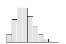
Lambda = 3
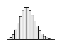
Lambda = 10


Describes the number of times an event occurs in a finite observation space. For example, a Poisson distribution can describe the number of defects in the mechanical system of an airplane or the number of calls to a call center. The Poisson distribution is often used in quality control, reliability/survival studies, and insurance.
The Poisson distribution is defined by one parameter: lambda. This parameter equals the mean and variance. As lambda increases, the Poisson distribution approaches a normal distribution.
|
Lambda = 3 |
Lambda = 10 |
|
|
|
A variable follows a Poisson distribution if the following conditions are met:
Another property of the Poisson distribution is the rate of occurrence, which equals the mean (lambda) divided by the dimension of your observation space. It is useful for comparing Poisson counts collected in different observation spaces. For example, Switchboard A receives 50 telephone calls in 5 hours, and Switchboard B receives 80 calls in 10 hours. You cannot directly compare these values because their observation spaces are different. You must calculate the occurrence rate to compare these counts. The rate for Switchboard A is (50 calls / 5 hours) = 10 calls/hour. The rate for Switchboard B is (80 calls / 8 hours) = 8 calls/hour.
The Poisson distribution is similar to the binomial distribution because they both model counts of events. However, within its finite observation space, the Poisson distribution places no upper bound on this count: a switchboard could receive an infinite number of calls in a day and not violate Poisson distribution requirements. Conversely, the binomial distribution does set an upper limit on the count: the number of events you observe cannot exceed the number of trials you perform.