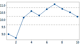
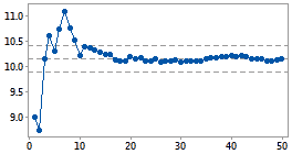
Cumulative %Defective plot

In capability analysis for binomial data, this graph helps verify that you have collected data from enough samples to calculate a stable estimate of the mean percentage of defective items (%Defective) in your process. This statistic is central to the capability study, so without sufficient data to estimate mean %Defective, the analysis cannot continue.

This graph plots the mean %Defective against the ordered samples to show how the estimate changes as you collect more samples. You can conclude that you have collected enough samples when the estimate levels off to a stable value. The plot also includes horizontal lines to represent the mean %Defective, calculated from all samples, and its upper and lower confidence bounds.

For example, you are studying workplace absenteeism at your company, so you observe the percentage of employees who are absent on 10 random days. Because absenteeism is a binary condition (absent or present), you analyze the data with binary capability analysis. The output includes the first plot of cumulative %Defective below. The estimate of %defective has not stabilized after ten samples, so you must collect more samples to continue the analysis. You repeat the study with data from 50 days and produce the second plot of cumulative %Defective below. It clearly shows the estimate of %Defective has reached a stable value. You conclude that 50 samples provide sufficient data to conduct your capability study, so you continue with the analysis.