main topic interpreting results session command see also
In the example for a linear response surface model, you determined that the linear model did not adequately represent the response surface. The next step is to fit the quadratic model. The quadratic model allows detection of curvature in the response surface.
To reduce the impact of non-orthogonal terms, Minitab fits the model in coded units.
1 Open the worksheet CCD_EX1.MTW. (The design and response data have been saved for you.)
2 Choose Stat > DOE > Response Surface > Analyze Response Surface Design.
3 In Responses, enter BeanYield.
4 Click Terms.
5 From Include the following terms, choose Full quadratic. Click OK.
6 Click Graphs.
7 Under Residual Plots, choose Four in one. Click OK in each dialog box.
Session window output
Response Surface Regression: BeanYield versus Nitrogen, PhosAcid, Potash
Analysis of Variance
Source DF Adj SS Adj MS F-Value P-Value Model 9 36.4653 4.0517 4.08 0.019 Linear 3 7.7886 2.5962 2.62 0.109 Nitrogen 1 4.4960 4.4960 4.53 0.059 PhosAcid 1 0.4593 0.4593 0.46 0.512 Potash 1 2.8332 2.8332 2.86 0.122 Square 3 13.3857 4.4619 4.50 0.030 Nitrogen*Nitrogen 1 6.5943 6.5943 6.65 0.027 PhosAcid*PhosAcid 1 4.5640 4.5640 4.60 0.058 Potash*Potash 1 1.0772 1.0772 1.09 0.322 2-Way Interaction 3 15.2909 5.0970 5.14 0.021 Nitrogen*PhosAcid 1 3.6721 3.6721 3.70 0.083 Nitrogen*Potash 1 11.1865 11.1865 11.28 0.007 PhosAcid*Potash 1 0.4325 0.4325 0.44 0.524 Error 10 9.9198 0.9920 Lack-of-Fit 5 7.3802 1.4760 2.91 0.133 Pure Error 5 2.5396 0.5079 Total 19 46.3851
Model Summary
S R-sq R-sq(adj) R-sq(pred) 0.995984 78.61% 59.37% 0.00%
Coded Coefficients
Term Effect Coef SE Coef T-Value P-Value VIF Constant 10.462 0.406 25.76 0.000 Nitrogen -1.148 -0.574 0.270 -2.13 0.059 1.00 PhosAcid 0.367 0.183 0.270 0.68 0.512 1.00 Potash 0.911 0.455 0.270 1.69 0.122 1.00 Nitrogen*Nitrogen -1.353 -0.676 0.262 -2.58 0.027 1.02 PhosAcid*PhosAcid 1.126 0.563 0.262 2.14 0.058 1.02 Potash*Potash -0.547 -0.273 0.262 -1.04 0.322 1.02 Nitrogen*PhosAcid -1.355 -0.678 0.352 -1.92 0.083 1.00 Nitrogen*Potash 2.365 1.182 0.352 3.36 0.007 1.00 PhosAcid*Potash 0.465 0.233 0.352 0.66 0.524 1.00
Regression Equation in Uncoded Units
BeanYield = 12.45 + 0.96 Nitrogen - 2.28 PhosAcid - 1.48 Potash - 0.268 Nitrogen*Nitrogen + 1.116 PhosAcid*PhosAcid - 0.239 Potash*Potash - 0.600 Nitrogen*PhosAcid + 0.695 Nitrogen*Potash + 0.306 PhosAcid*Potash
Fits and Diagnostics for Unusual Observations
Obs BeanYield Fit Resid Std Resid 2 11.060 12.362 -1.302 -2.09 R 7 8.260 9.514 -1.254 -2.01 R 16 13.190 12.004 1.186 2.07 R
R Large residual |
Graph window output

Because the linear model suggested that a higher-order model is needed to adequately model the response surface, you fit the full quadratic model. For the full quadratic model, the p-value for lack of fit is 0.133 suggesting that this model adequately fits the data.
The Analysis of Variance table summarizes the linear terms, the squared terms, and the interactions. The small p-values for the interactions (p = 0.021) and the squared terms (p = 0.030) suggest there is curvature in the response surface. Small p-values for the Nitrogen by Potash interaction (p = 0.007), Nitrogen squared (p = 0.027), and Phosphoric acid squared (p = 0.058) indicate that these effects are statistically significant.
The coefficient table gives the coefficients for all the terms in the model. Because you used an orthogonal design, each effect is estimated independently. Therefore, the coefficients for the linear terms are the same as when you fit just the linear model. The error term, s = 0.995984, is smaller because you reduced the variability accounted for by error.
The VIFs are all close to 1, which indicates that the predictors are not correlated. VIF values greater than 5-10 suggest that the regression coefficients are poorly estimated due to severe multicollinearity.
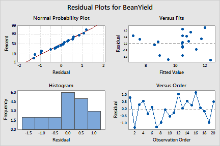
In addition, Minitab draws four residual plots. The residual plots do not indicate any problems with the model. For assistance in interpreting residual plots, see Residual plot choices.
For contour and surface plots of this response surface, see Example of a Contour Plot and a Surface Plot.