main topic interpreting results session command see also
Suppose you work for a company that manufactures engine windings for turbine assemblies. Engine windings may decompose at an unacceptable rate at high temperatures. You want to know, at given high temperatures, at what time do 1% of the engine windings fail. You plan to get this information by using Parametric Distribution Analysis (Right Censoring), but you first want to have a quick look at your data from different perspectives.
First you collect data for times to failure for the engine windings
at two temperatures. In the first sample, you test 50 windings at 80
1 Open the worksheet RELIABLE.MTW.
2 Choose Stat > Reliability/Survival > Distribution Analysis (Right Censoring) > Distribution Overview Plot.
3 In Variables, enter Temp80 and Temp100.
4 In Distribution, choose Lognormal.
5 Click Censor. Choose Use censoring columns and enter Cens80 and Cens100. Click OK in each dialog box.
Session window output
Distribution Overview Plot: Temp80, Temp100
Results for variable: Temp80
Goodness-of-Fit
Anderson-Darling Distribution (adj) Lognormal 67.800
Results for variable: Temp100
Goodness-of-Fit
Anderson-Darling Distribution (adj) Lognormal 17.253
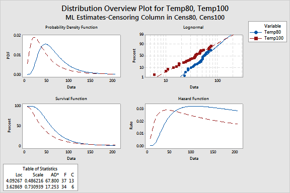
Distribution Overview Plot for Temp80, Temp100 |
Graph window output

These four plots describe the failure rate of engine windings at two
different temperatures. With these plots, you can determine how much more
likely it is that engine windings will fail when running at 100