main topic interpreting results session command see also
You want to determine the shelf life for pills that contain a new drug. The concentration of the drug in the pills decreases over time. You want to determine when the pills reach 90% of the intended concentration.
You create 5 batches of the medication and test one pill from each batch at 9 different times. In Example of Creating a Stability Study Worksheet, you created a data collection worksheet for this study.
1 Open the worksheet SHELFLIFE.MTW.
2 Choose Stat > Regression > Stability Study > Stability Study.
3 In Response, enter Drug%.
4 In Time, enter Month.
5 In Batch, enter Batch.
6 In Lower spec, type 90.
7 Click Graphs.
8 Under Shelf life plot, in the second drop-down list, choose No graphs for individual batches.
9 Under Residual Plots, choose Four in one.
10 Click OK in each dialog box.
Session window output
Stability Study: Drug% versus Month, Batch
Method
Rows unused 5
Factor Information
Factor Type Number of Levels Levels Batch Fixed 5 1, 2, 3, 4, 5
Model Selection with α = 0.25
Source DF Seq SS Seq MS F-Value P-Value Month 1 122.460 122.460 345.93 0.000 Batch 4 2.587 0.647 1.83 0.150 Month*Batch 4 3.850 0.962 2.72 0.048 Error 30 10.620 0.354 Total 39 139.516
Terms in selected model: Month, Batch, Month*Batch
Model Summary
S R-sq R-sq(adj) R-sq(pred) 0.594983 92.39% 90.10% 85.22%
Coefficients
Term Coef SE Coef T-Value P-Value VIF Constant 100.085 0.143 701.82 0.000 Month -0.13633 0.00769 -17.74 0.000 1.07 Batch 1 -0.232 0.292 -0.80 0.432 3.85 2 0.068 0.292 0.23 0.818 3.85 3 0.394 0.275 1.43 0.162 3.41 4 -0.317 0.292 -1.08 0.287 3.85 5 0.088 0.275 0.32 0.752 * Month*Batch 1 0.0454 0.0164 2.76 0.010 4.52 2 -0.0241 0.0164 -1.47 0.152 4.52 3 -0.0267 0.0136 -1.96 0.060 3.65 4 0.0014 0.0164 0.08 0.935 4.52 5 0.0040 0.0136 0.30 0.769 *
Regression Equation
Batch 1 Drug% = 99.853 - 0.0909 Month
2 Drug% = 100.153 - 0.1605 Month
3 Drug% = 100.479 - 0.1630 Month
4 Drug% = 99.769 - 0.1350 Month
5 Drug% = 100.173 - 0.1323 Month
Fits and Diagnostics for Unusual Observations
Obs Drug% Fit Resid Std Resid 11 98.001 99.190 -1.189 -2.21 R 43 92.242 92.655 -0.413 -1.47 X 44 94.069 93.823 0.246 0.87 X
R Large residual X Unusual X
Shelf Life Estimation
Lower spec limit = 90 Shelf life = time period in which you can be 95% confident that at least 50% of response is above lower spec limit
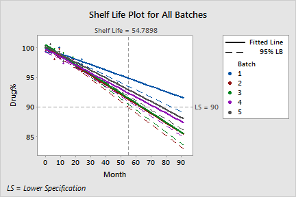
Batch Shelf Life 1 83.552 2 54.790 3 57.492 4 60.898 5 66.854 Overall 54.790 |
Graph window output


For the pill data, the p-value for the Month by Batch interaction (Month*Batch) is 0.048. Because the p-value is less than the a-level of 0.25, the model cannot be reduced.
Both Month and the Month by Batch interaction are significant. Thus the regression equations for each batch have different intercepts and slopes. Batch 3 has the steepest slope, -0.1630, which indicates that, each month, the concentration of medication (Drug%) for Batch 3 decreases 0.163 percentage points. Batch 4 has the smallest intercept, 99.769, which indicates that Batch 4 had the lowest concentration at time zero.
Minitab displays the shelf life estimates for each batch. The shortest shelf life estimate is 54.79 months, so the overall shelf life for the product is estimated as 54.79 months.
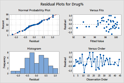
The residuals appear to be reasonably normal and randomly scattered about zero. There are more points on the right side of the residuals versus fits plot than on the left. This pattern occurs because more observations were collected earlier in the study, when drug concentrations were high.