main topic interpreting results session command see also
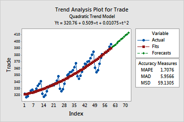
You collect employment data in a trade business over 60 months and wish to predict employment for the next 12 months. Because there is an overall curvilinear pattern to the data, you use trend analysis and fit a quadratic trend model. Because there is also a seasonal component, you save the fits and residuals to perform decomposition of the residuals (see Example of Decomposition).
1 Open the worksheet EMPLOY.MTW.
2 Choose Stat > Time Series > Trend Analysis.
3 In Variable, enter Trade.
4 Under Model Type, choose Quadratic.
5 Check Generate forecasts and enter 12 in Number of forecasts.
6 Click Storage.
7 Check Fits (Trend Line), Residuals (detrended data), and Forecasts. Click OK in each dialog box.
Session Window Output
Trend Analysis for Trade
Data Trade Length 60 NMissing 0
Fitted Trend Equation
Yt = 320.76 + 0.509×t + 0.01075×t^2
Accuracy Measures
MAPE 1.7076 MAD 5.9566 MSD 59.1305
Forecasts
Period Forecast 61 391.818 62 393.649 63 395.502 64 397.376 65 399.271 66 401.188 67 403.127 68 405.087 69 407.068 70 409.071 71 411.096 72 413.142 |
Graph window output

The trend plot that shows the original data, the fitted trend line, and forecasts. The Session window output also displays the fitted trend equation and three Measures of Accuracy to help you determine the accuracy of the fitted values: MAPE, MAD, and MSD. The trade employment data show a general upward trend, though with an evident seasonal component. The trend model appears to fit well to the overall trend, but the seasonal pattern is not well fit. To better fit these data, you also use decomposition on the stored residuals and add the trend analysis and decomposition fits and forecasts (see Example of decomposition).