main topic interpreting results session command see also
You wish to predict trade employment for the next 12 months using data collected over 60 months. Because the data have a trend that is fit well by trend analysis' quadratic trend model and possess a seasonal component, you use the residuals from trend analysis example (see Example of a trend analysis) to combine both trend analysis and decomposition for forecasting.
1 Do the trend analysis example.
2 Choose Stat > Time Series > Decomposition.
3 In Variable, enter the name of the residual column you stored in the trend analysis.
4 In Seasonal length, enter 12.
5 Under Model Type, choose Additive. Under Model Components, choose Seasonal only.
6 Check Generate forecasts and enter 12 in Number of forecasts.
7 Click Storage. Check Forecasts and Fits.
8 Click OK in each dialog box.
Session window output
Trend Analysis for Trade
Data Trade Length 60 NMissing 0
Fitted Trend Equation
Yt = 320.76 + 0.509×t + 0.01075×t^2
Accuracy Measures
MAPE 1.7076 MAD 5.9566 MSD 59.1305
Forecasts
Period Forecast 61 391.818 62 393.649 63 395.502 64 397.376 65 399.271 66 401.188 67 403.127 68 405.087 69 407.068 70 409.071 71 411.096 72 413.142
Time Series Decomposition for RESI1
Additive Model
Data RESI1 Length 60 NMissing 0
Seasonal Indices
Period Index 1 -8.4826 2 -13.3368 3 -11.4410 4 -5.8160 5 0.5590 6 3.5590 7 1.7674 8 3.4757 9 3.2674 10 5.3924 11 8.4965 12 12.5590
Accuracy Measures
MAPE 881.582 MAD 2.802 MSD 11.899
Forecasts
Period Forecast 61 -8.4826 62 -13.3368 63 -11.4410 64 -5.8160 65 0.5590 66 3.5590 67 1.7674 68 3.4757 69 3.2674 70 5.3924 71 8.4965 72 12.5590 |
Graph window output


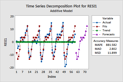
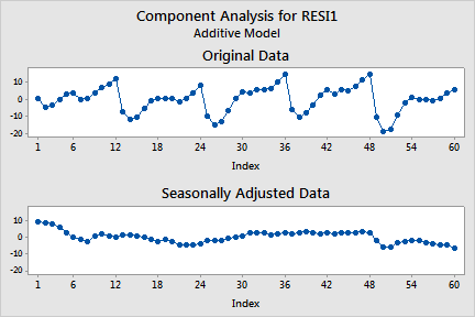
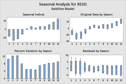
Decomposition generates three sets of plots:
In addition, Minitab displays the fitted trend line, the seasonal indices, the three accuracy measures- MAPE, MAD, and MSD (see Measures of accuracy) - and forecasts in the Session window.
In the example, the first graph shows that the detrended residuals from trend analysis are fit fairly well by decomposition, except that part of the first annual cycle is underpredicted and the last annual cycle is overpredicted. This is also evident in the lower right plot of the second graph; the residuals are highest in the beginning of the series and lowest at the end.