main topic interpreting results session command see also
You wish to predict employment for the next six months in a food preparation industry using data collected over the last 60 months. You use Winters' method with the default multiplicative model, because there is a seasonal component, and possibly trend, apparent in the data.
1 Open the worksheet EMPLOY.MTW.
2 Choose Stat > Time Series > Winters' Method.
3 In Variable, enter Food. In Seasonal length, enter 12.
4 Under Model Type, choose Multiplicative.
5 Check Generate forecasts and enter 6 in Number of forecasts. Click OK.
Session window output
Winters’ Method for Food
Multiplicative Method
Data Food Length 60
Smoothing Constants
α (level) 0.2 γ (trend) 0.2 δ (seasonal) 0.2
Accuracy Measures
MAPE 1.88377 MAD 1.12068 MSD 2.86696
Forecasts
Period Forecast Lower Upper 61 57.8102 55.0646 60.5558 62 57.3892 54.6006 60.1778 63 57.8332 54.9966 60.6698 64 57.9307 55.0414 60.8199 65 58.8311 55.8847 61.7775 66 62.7415 59.7339 65.7492 |
Graph window output

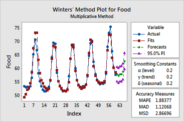
Minitab generated the default time series plot which displays the series and fitted values (one-period-ahead forecasts), along with the six forecasts.
In both the Session and Graph windows, Minitab displays the smoothing constants (weights) used for level, trend, and seasonal components used and three measures to help you determine the accuracy of the fitted values: MAPE, MAD, and MSD (see Measures of accuracy).
For these data, MAPE, MAD, and MSD were 1.88, 1.12, and 2.87, respectively, with the multiplicative model. MAPE, MAD, and MSD were 1.95, 1.15, and 2.67, respectively (output not shown) with the additive model, indicating that the multiplicative model provided a slightly better fit according to two of the three accuracy measures.