main topic interpreting results session commands see also
Suppose you work for a company that manufactures floor tiles, and are concerned about warping in the tiles. To ensure production quality, you measured warping in 10 tiles each working day for 10 days. The distribution of the data is unknown. Individual Distribution Identification allows you to fit these data with 14 parametric distributions and 2 transformations.
1 Open the worksheet TILES.MTW.
2 Choose Stat > Quality Tools > Individual Distribution Identification.
3 Under Data are arranged as, choose Single column, then enter Warping.
4 Choose Use all distributions and transformations. Click OK.
Session window output
Distribution ID Plot for Warping
Descriptive Statistics
N N* Mean StDev Median Minimum Maximum Skewness Kurtosis 100 0 2.92307 1.78597 2.60726 0.28186 8.09064 0.707725 0.135236
Box-Cox transformation: λ = 0.5
Johnson transformation function: 0.882908 + 0.987049 × Ln( ( X + 0.132606 ) / ( 9.31101 - X ) )
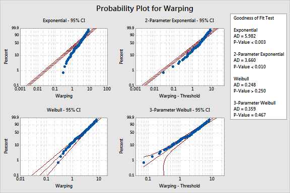
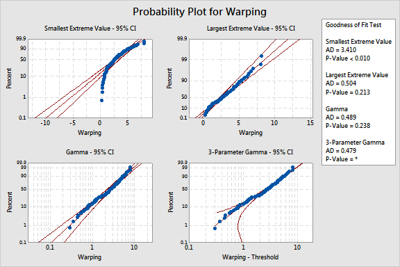
Goodness of Fit Test
Distribution AD P LRT P Normal 1.028 0.010 Box-Cox Transformation 0.301 0.574 Lognormal 1.477 <0.005 3-Parameter Lognormal 0.523 * 0.007 Exponential 5.982 <0.003 2-Parameter Exponential 3.660 <0.010 0.000 Weibull 0.248 >0.250 3-Parameter Weibull 0.359 0.467 0.225 Smallest Extreme Value 3.410 <0.010 Largest Extreme Value 0.504 0.213 Gamma 0.489 0.238 3-Parameter Gamma 0.479 * 1.000 Logistic 0.879 0.013 Loglogistic 1.239 <0.005 3-Parameter Loglogistic 0.692 * 0.085 Johnson Transformation 0.231 0.799
ML Estimates of Distribution Parameters
Distribution Location Shape Scale Threshold Normal* 2.92307 1.78597 Box-Cox Transformation* 1.62374 0.53798 Lognormal* 0.84429 0.74444 3-Parameter Lognormal 1.37877 0.41843 -1.40015 Exponential 2.92307 2-Parameter Exponential 2.66789 0.25518 Weibull 1.69368 3.27812 3-Parameter Weibull 1.50491 2.99693 0.20988 Smallest Extreme Value 3.86413 1.99241 Largest Extreme Value 2.09575 1.41965 Gamma 2.34280 1.24768 3-Parameter Gamma 2.38984 1.23136 -0.01968 Logistic 2.79590 1.01616 Loglogistic 0.90969 0.42168 3-Parameter Loglogistic 1.30433 0.26997 -1.09399 Johnson Transformation* 0.01120 0.99495
* Scale: Adjusted ML estimate |
Graph window output


Minitab displays descriptive statistics, goodness-of-fit test results, and probability plots.
Descriptive statistics - The table of descriptive statistics provides you with summary information for the whole column of data. All the statistics are based on the non-missing (N = 100) values. For these data, m = 2.92307 and s = 1.78597.
Transformations - The Box-Cox transformations uses a lambda of 0.05 and the Johnson transformation function is 0.882908 + 0.987049 * ln((X + 0.132606) / (9.31101 - X)).
Goodness-of-fit test - The table includes Anderson-Darling (AD) statistics and the corresponding p-value for a distribution. For a critical value a, a p-value greater than a suggests that the data follow that distribution. Minitab also includes a p-value for Likelihood ratio test (LRT P), which tests whether a 2-parameter distribution would fit the data equally well compared to its 3-parameter counterpart.
The p-values of >0.25, 0.467, 0.213, and 0.238 indicate that the Weibull, 3-parameter Weibull, largest extreme value, and gamma distributions fit the data well. The Box-Cox (p-value = 0.574) and Johnson transformations (p-value = 0.799) also provide good fits for the data.
Use the LRT P value to determine whether the corresponding 3-parameter distribution improves the fit over the 2-parameter distribution. The LRT P value of 0.225 suggests that the 3-parameter Weibull distribution does not significantly improve the fit compared to the 2-parameter Weibull distribution. The LRT P value of 1.000 suggests that the 3-parameter gamma distribution does not significantly improve the fit compared to the 2-parameter gamma distribution. However, the 3-parameter lognormal improves the fit over the 2-parameter lognormal (LRT P = 0.007) and the 2-parameter exponential improves the fit over the exponential (LRT P = 0.000).
Probability plot - The probability plot includes percentile points for corresponding probabilities of an ordered data set. The middle line is the expected percentile from the distribution based on maximum likelihood parameter estimates. The left and right line represent the lower and upper bounds for the confidence intervals of each percentile.
The probability plots shows that the data points fall approximately on a straight line and within the confidence intervals for the 2-parameter Weibull, 3-parameter Weibull, largest extreme value, and gamma distribution.
If more than one distribution fits your data, see selecting a distribution for guidance. If both normal and nonnormal models fit the data about the same, it is probably better to choose the normal model, since it provides estimates of both overall and within process capability. For other example using these data, see Example of Capability Analysis for Nonnormal Data and Example of Capability Analysis using a Box-Cox Transformation.