main topic interpreting results session command see also
In Example of a stability study, you determined the shelf life of a new medication using the default method, which treats batch as a fixed factor. If you choose batches randomly from a larger population of possible batches, then you can analyze batch as a random factor.
For this example, suppose that you want to calculate shelf life for a medication. You randomly select 8 batches of medication from a larger population of possible batches.
1 Open the worksheet SHELFLIFERANDOM.MTW.
2 Choose Stat > Regression > Stability Study > Stability Study.
3 In Response, enter Drug%.
4 In Time, enter Month.
5 In Batch, enter Batch.
6 In Lower spec, type 90.
7 Click Options.
8 Choose Batch is a random factor.
9 Click OK and then click Graphs.
10 Under Residual Plots, choose Four in one.
11 Click OK in each dialog box.
Session window output
Stability Study: Drug% versus Month, Batch
Factor Information
Factor Type Number of Levels Levels Batch Random 8 1, 2, 3, 4, 5, 6, 7, 8
Model Selection with α = 0.25
Model -2 LogLikelihood Difference P-Value Month Batch Month*Batch 128.599 Month Batch 133.424 4.82476 0.059
Terms in selected model: Month, Batch, Month*Batch
Variance Components
Source Var % of Total SE Var Z-Value P-Value Batch 0.527403 72.91% 0.303847 1.735755 0.041 Month*Batch 0.000174 0.02% 0.000142 1.224106 0.110 Error 0.195740 27.06% 0.036752 5.325920 0.000 Total 0.723317
Model Summary
S R-sq R-sq(adj) 0.442425 96.91% 96.87%
Coefficients
Term Coef SE Coef DF T-Value P-Value Constant 100.060247 0.268705 7.22 372.380078 0.000 Month -0.138766 0.005794 7.22 -23.950307 0.000
Random Effect Predictions
Term BLUP StDev DF T-Value P-Value Batch 1 1.359433 0.313987 12.45 4.329582 0.001 2 0.395376 0.313987 12.45 1.259213 0.231 3 0.109150 0.313987 12.45 0.347625 0.734 4 -0.409321 0.313987 12.45 -1.303625 0.216 5 -0.135643 0.313987 12.45 -0.432002 0.673 6 -1.064735 0.313987 12.45 -3.391015 0.005 7 0.049419 0.313987 12.45 0.157391 0.877 8 -0.303678 0.313987 12.45 -0.967169 0.352 Month*Batch 1 0.006281 0.008581 10.49 0.731927 0.480 2 0.019905 0.008581 10.49 2.319532 0.042 3 -0.013831 0.008581 10.49 -1.611737 0.137 4 0.003468 0.008581 10.49 0.404171 0.694 5 0.001240 0.008581 10.49 0.144454 0.888 6 0.000276 0.008581 10.49 0.032141 0.975 7 -0.010961 0.008581 10.49 -1.277269 0.229 8 -0.006378 0.008581 10.49 -0.743220 0.474
Marginal Fits and Diagnostics for Unusual Observations
Obs Drug% Fit DF Resid Std Resid 10 101.564000 99.643950 7.04383 1.920050 2.37526 R 31 100.618000 98.811354 7.05287 1.806646 2.21379 R 55 98.481000 96.729866 8.87399 1.751134 2.03349 R
R Large residual
Shelf Life Estimation
Lower spec limit = 90 Shelf life = time period in which you can be 95% confident that at least 95% of response is above lower spec limit
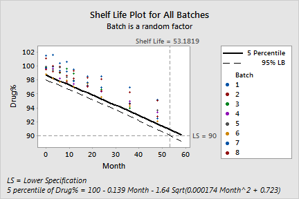
Shelf life for all batches = 53.1819 |
Graph window output


In the model selection process, Minitab compares the full model, "Month Batch Month*Batch", to the model that does not include the interaction term. Because the p-value for that comparison (0.059) is less than a (0.25), the interaction term cannot be removed from the model. The final model includes Month, Batch, and the Month by Batch interaction (Month*Batch).
When the batch factor is random, Minitab calculates shelf life based on the 95th percentile rather than the 50th percentile. (You can change this setting, and the value of alpha, in the Options subdialog box.) Shelf life is the time at which you can no longer be 95% confident that at least 95% of the response is within your specification limits. The shelf life for the present data is approximately 53.18 months.
The coefficients table shows the estimated coefficients for the fixed effects in the model. These coefficients are the intercept (Constant) and the slope (Month) for the marginal fitted equation (shown below), which predicts the fitted value for any random batch.
Drug% = 100.06 - 0.13877 Month
The table of random effect predictions shows the predicted values for the random terms. With these predicted values, you can determine the intercept and the slope for the conditional fitted equations, which predict the fitted values for the specific batches. (You can view these equations using Minitab's Predict feature.) For example, the intercept for Batch 1 is 101.359, which is equal to the Constant (100.06) plus the best linear unbiased predicted value (BLUP) for Batch 1 (1.359). The slope for Batch 1 is - 0.13248, which is equal to Month (-0.138766) plus the BLUP for Batch 1 by Month (0.006281).
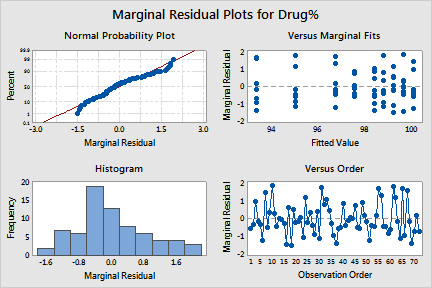
The marginal residual plots for Drug% (above) show that the marginal residuals may not be normally distributed with constant variance. The histogram is flatter than the normal distribution, and the points in the normal probability plot do not follow the line well. One reason for the nonnormal behavior of the marginal residuals is that, when the final model includes the batch by time interaction, the variance of the marginal residuals depends on the time variable and may not be constant.
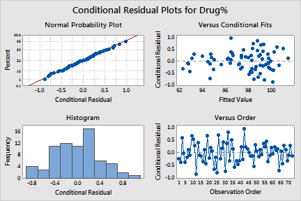
You can use the conditional residuals to check the normality of the error term in the model.
1 Press CTRL+E or choose Stat > Regression > Stability Study > Stability Study.
2 Click Graphs.
3 In Residuals for plots, choose Conditional regular.
4 Click OK in each dialog box.
Graph window output

The conditional residuals appear to be normally distributed. The full model appears to fit the data well.