main topic interpreting results session command see also
You wish to predict employment over 6 months in a segment of the metals industry using data collected over 60 months. You use single exponential smoothing because there is no clear trend or seasonal pattern in the data.
1 Open the worksheet EMPLOY.MTW.
2 Choose Stat > Time Series > Single Exp Smoothing.
3 In Variable, enter Metals.
4 Check Generate forecasts, and enter 6 in Number of forecasts. Click OK.
Session window output
Single Exponential Smoothing for Metals
Data Metals Length 60
Smoothing Constant
α 1.04170
Accuracy Measures
MAPE 1.11648 MAD 0.50427 MSD 0.42956
Forecasts
Period Forecast Lower Upper 61 48.0560 46.8206 49.2914 62 48.0560 46.8206 49.2914 63 48.0560 46.8206 49.2914 64 48.0560 46.8206 49.2914 65 48.0560 46.8206 49.2914 66 48.0560 46.8206 49.2914 |
Graph window output

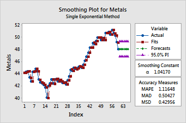
Minitab generated the default time series plot which displays the series and fitted values (one-period-ahead forecasts), along with the six forecasts.
In both the Session and Graph windows, Minitab displays the smoothing constant (weight) used and three measures to help you to determine the accuracy of the fitted values: MAPE, MAD, and MSD (see Measures of accuracy). The three accuracy measures, MAPE, MAD, and MSD, were 1.12, 0.50, and 0.43, respectively for the single exponential smoothing model, compared to 1.55, 0.70, and 0.76, respectively, for the moving average fit (see Example of moving average). Because these values are smaller for single exponential smoothing, you can judge that this method provides a better fit to these data.