main topic interpreting results session command see also
You wish to predict employment over the next 6 months in a segment of the metals industry using data collected over 60 months. You use the moving average method as there is no well-defined trend or seasonal pattern in the data.
1 Open the worksheet EMPLOY.MTW.
2 Choose Stat > Time Series > Moving Average.
3 In Variable, enter Metals. In MA length, enter 3.
4 Check Center the moving averages.
5 Check Generate forecasts, and enter 6 in Number of forecasts. Click OK.
Session window output
Moving Average for Metals
Data Metals Length 60 NMissing 0
Moving Average
Length 3
Accuracy Measures
MAPE 0.890317 MAD 0.402299 MSD 0.255287
Forecasts
Period Forecast Lower Upper 61 49.2 48.2097 50.1903 62 49.2 48.2097 50.1903 63 49.2 48.2097 50.1903 64 49.2 48.2097 50.1903 65 49.2 48.2097 50.1903 66 49.2 48.2097 50.1903 |
Graph window output

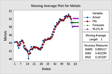
Minitab generated the default time series plot which displays the series and fitted values (one-period-ahead forecasts), along with the six forecasts. Notice that the fitted value pattern lags behind the data pattern. This is because the fitted values are the moving averages from the previous time unit. If you wish to visually inspect how moving averages fit your data, plot the smoothed values rather than the predicted values.
To see exponential smoothing methods applied to the same data, see Example of single exponential smoothing and Example of double exponential smoothing.
In the Session window, Minitab displays three measures to help you determine the accuracy of the fitted values: MAPE, MAD, and MSD. See Measures of accuracy. Minitab also displays the forecasts along with the corresponding lower and upper 95% prediction limits.
| Minitab help | Stat | Graph | SixSigma | DOE | Glossary | Reliability | SPC,MSA,CPK | ||
|
|||||||||