Example of analyzing variability
main topic     interpreting results     session command     see also 

In the Example of preprocessing responses, you performed a 2-level factorial experiment with 8 repeats to investigate how three variables-reaction time, reaction temperature, and type of catalyst-affect the variability of the yield. Use Analyze Variability to determine which terms (main effects and two-way interactions) are significantly related to differences in the variability of yield. Before you can analyze the variability of this data, you must first do the Example of preprocessing responses to store the standard deviations and number of replicates of the response.

The analysis for this example is performed in two steps. In the first step, you use least squares regression to fit and reduce the model. Once you identify an appropriate reduced model, in step two, analyze the reduced model using maximum likelihood estimation to obtain the final model coefficients.

Step 1: Analyze the design using least squares regression estimation

1    Complete the Example of preprocessing responses.

2    Choose Stat > DOE > Factorial > Analyze Variability.

3    In Response (standard deviations), enter StdYield.

4    Click Terms.

5    In Include terms from the model up through order, choose 2 from the drop-down list. Click OK.

6    Click Graphs. Under Effects Plots, check Pareto, Normal, and Half Normal. Click OK in each dialog box.

Session window output

Graph window output

Interpreting the Results

In the first step of the analysis, you used least squares regression to fit the model. One approach to analyzing the variability of data is to use least squares regression to determine which factors are significantly related to the response. Once a reduced model is identified, use maximum likelihood estimation (MLE) to determine the final model coefficients. If you have terms that are borderline significant, you may want to examine both the regression and MLE results to determine which factors to retain in your model. See [7] for more information. In many cases, the differences between the least squares and MLE results are minor.

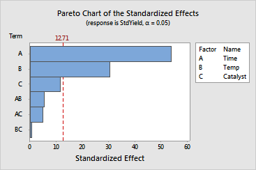
For this example, the analysis of variance table provides a summary of the main effects and interactions. Look at the p-values to determine whether or not you have any significant effects.

The results indicate that time and temperature are significant at the 0.05 a-level. The variable catalyst is almost significant at the 0.05 a-level. The interactions are not significant at the 0.05 a-level. As you reduce the model, the p-values change.

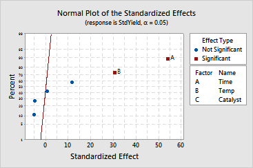
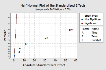
The normal, half normal, and Pareto plots of the effects allow you to visually identify the important effects and compare the relative magnitude of the various effects. The plots confirm that time and temperature are significant at the 0.05 a-level.

At this point, you should reduce the model using the least squares regression method to determine which terms to retain in the model. For the purposes of this example, the model with time, temperature, catalyst, time by temperature, and time by catalyst is used as the reduced model. This model is just one of the possible reduced models you could have chosen. In practice, you may need to fit several models to find the appropriate model. Stepwise variable selection can help you to look at several models.

Step 2: Analyze the reduced model using maximum likelihood estimation

1    Choose Stat > DOE > Factorial > Analyze Variability.

2    In Response (standard deviations), enter StdYield.

3    Click Options.

4    Under Estimation method, choose Maximum likelihood. Click OK.

5    Click Terms.

6    Move BC from Selected Terms to Available Terms. Click OK.

7    Click Graphs.

8    Under Effects Plots, uncheck Pareto, Normal, and Half Normal.

9    Under Residual Plots, click Three in one.

10    Click OK in each dialog box.

Session window output

Graph window output

Interpreting the Results

After choosing an appropriate reduced model using least squares estimation, you refit the model using maximum likelihood estimation to obtain the most precise effects and coefficients. The results indicate that:

·    Time has the strongest effect at 2.0365. The ratio effect indicates that the standard deviation increases by a factor of 7.6636 when time is changed from the low to high level.

·    Temperature has the next strongest effect at 1.1491. The ratio effect indicates that the standard deviation increases by a factor of 3.1552 when temperature is changed from the low to high level.

·    Catalyst has the smallest main effect at .4300. The ratio effect indicates that the standard deviation increases by a factor of 1.5373 when catalyst is changed from the low to high level.

The interactions are not statistically significant at the 0.05 a-level. The interactions remain in the model because the p-values from the least squares estimation are more reliable.

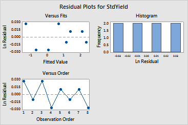
The residuals plots show no evidence of patterns or outliers.